GIS Lab 4
Goal and Background:
The goal for this lab was to be able to better develop our skills of composing query expressions to extract specific data from the databases we were provided with. We were to compose five different multiple criteria queries over the course of this lab, each of which would assess our knowledge of attribute and spatial queries and how to assess the results that come from the two.
Methods:
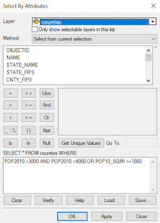
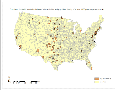
To begin, I started with a blank map and added the counties data located in USA mgisdata. For the first question I wrote a multiple criteria query from counties with a population between 3000 and 4000 people in 2010 and also all counties in 2010 that had a population density of at least 1000 persons per square mile. My query for this is demonstrated in Figure 1. I got this because if you want all of the population between 3000 and 4000 and also all of the counties that had a population density of at least 1000 person per square mile you use OR and not AND. To answer how many counties met the above criteria, how many states me the criteria above, which state has the highest number of counties, and which state had 8 counties that met the criteria; I used the information in the attribute table I got from doing the query itself. From there I created a cartographically pleasing map to show the results from that query.
 |
| Figure 1: Multiple criteria query for Question 1 |
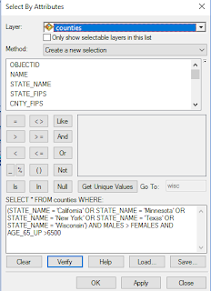
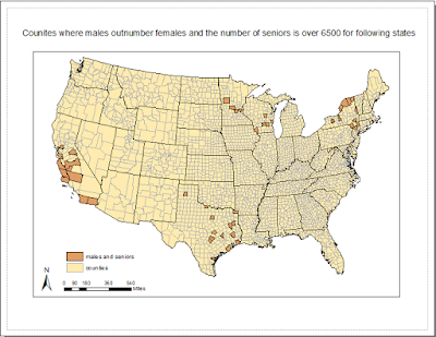
For question 2 I wrote a multiple criteria query for counties in Wisconsin, Texas, New York, Minnesota, and California where the male population is greater than the female population and also for these states where the number of seniors is above 6500. The query I wrote is in Figure 2 below. I got this because it asked for all of the states so I put OR in between all of the states names, and then AND in between the other information because we just want the data that overlaps the counties in those particular states. I then used the attribute table from counties that I got from the query to answer the specific questions the records. And then, created a cartographically pleasing map shows the counties that the query represented.
 |
| Figure 2: Multiple criteria query for Question 2 |
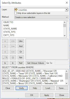
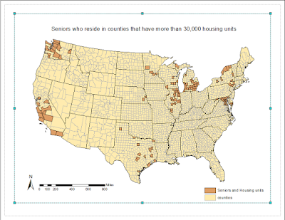
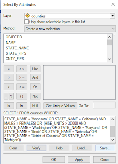
For question 3 I wrote a multiple criteria query developed from the second question just modified. What was added to this query was all other seniors in Washington, Maryland, Illinois, Nebraska, District of Columbia, and Michigan who reside in counties that have more than 30,000 housing units. The resulting query is shown in Figure 3 and 3.1. This was modified from the query in question two by moving senior age range to the top, followed by the original states, then males greater than females which were all combined by AND, then I followed that with OR and the new housing unit information and the new states added in this question. After finishing the query I again used the attribute table in counties to answer the new question from this query, and then made a cartographically pleasing map to show the new query.
 |
| Figure 3: First part of query for Question 3 |
 |
| Figure 3.1: Second part of query for Question 3 |
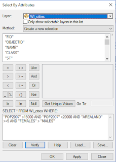
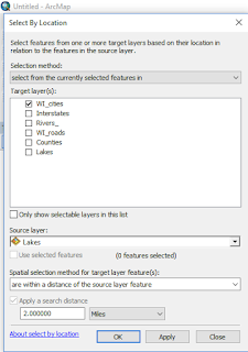
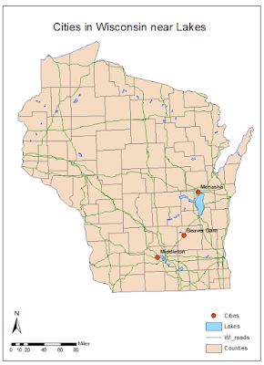
In part 2 I first had to download and unzip the Wisconsin Data set information provided to us by Dr. Cyril Wilson to be able to work on questions four and five. For question 4 I wrote a query for cities in Wisconsin with a 2007 population between 15,000 and 20,000, area of the city is at least 5 square miles in land area and also female population is greater than males, and also the cities are within 2 miles of a lake. The result of this query is in figure 4 below. I did AND in between all of the information because we just wanted the data that crossed over all of it. You can't do an attribute query for distance from a lake, so for that I did a spatial query shown in figure 4.1 below. I then was able to answer the following questions from the attribute table and spatial query, and then again created a cartographically pleasing map of the cities that were recorded.
 |
| Figure 4: Multiple criteria query for Question 4 |
 |
| Figure 4.1: Spatial query for Question 4 |
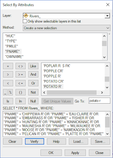
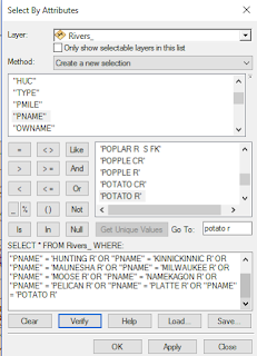
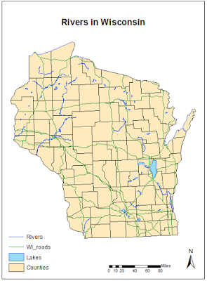
Finally, for question 5 I created a multiple criteria query from the following rivers in Wisconisn; Chippewa, Eau Claire, Embarrasss, Fisher, Hunting, Kinnickinnic, Maunesha, Milwaukee, Moose, Namekagon, Pelican, Platte, and Potato. The results are in Figures 5 and 5.1. Then in order to answer the questions about the records which included the total length of the the record of rivers from the query I had to create a new field in the Rivers attribute table. I then in that new field calculated the geometry in miles, and checked the Statistics bottom after to find the sum length in miles of all the rivers. Then created one last map of the resulted records found by this query.
 |
| Figure 5: Start of query for Question 5 |
 |
| Figure 5.1: End of query for Question 5 |
Results: In this results section I will be showing the final cartographically pleasing maps that are a result of the multiple criteria queries.
 |
| Figure 1.1: Map of query from question 1 |
 |
| Figure 2.1: Map of query from Question 2 |
 |
| Figure 3.2: Map of query from Question 3 |
 |
| Figure 4.2: Map of query from Question 4 |
 |
| Figure 5.2: Map of query from Question 5 |
Sources:
USA geodatabase data from the mgisdata from the Price book
Wisconsin cities, interstates, rivers, and counties shape files are from ESRI, 2011
Wisconsin Lakes created by Dr. Wilson 2012
