GIS Lab 5

Lab 5: Vector Geo-processing

Goal and Background: The goal of this lab is to be able to choose appropriate vector geoprocessing tools that we have discussed in class and used in our various tutorials. Using these skills to figure out an appropriate habitat for bears in Marquette County, Michigan which is the area of study. Another major goal is to become familiar with scripting in python while using geoprocessing tools to be able to prepare us for python programming in more advanced program.

Methods: I first unzipped the data from the Michigan Department of Natural Resources provided to us on D2L.
Part 1: In ArcCatolog for task one, I then created a feature class from the XY table by right clicking on the bear_locations_geog$ excel sheet and named in bear locations. From ArcMap I added all the bear management feature classes to a blank map, and also added the new feature class bear locations I made previously. After adding the feature class land-cover I changed the symbology to unique value of "minor type" to a multi-color scale. Then to find out what land cover type the bears were located in when their position was recorded with GPS by performing intersection to create a new feature class which has the ID number of the bear and the land cover type named bear_cover. Another second spatial operation was also necessary to find out how many bears were found in each habit type. Then to answer the questions in Objective 3, I used select by location to find the bears within 500 meters of a stream. For Objective 4 which was to find suitable land for bears in Marquette County, I used buffer for 500 metes within a stream, and then used select by attribute to select Mixed Forest Land, Forested Wetlands, and Evergreen Forest Land from the feature class landcover. I then intersected the two, to find the area that they both had in common and then dissolved the results to make the lines within the new feature class go away. For Objective 5, we were asked to find the suitable land for bears which is also within the DNR management lands of Michigan. I did this by intersecting the results form Objective 4 for suitable bear habitat with the feature class dnr_mgmt, and then using the dissolve tool to eliminate internal boundaries. Objective 6 asked to use the area in Objective 5, but make it so that it is not within 5 kilometers of any Urban or Built up lands. I did this in three steps by first using select by attributes to to select Urban or Built up lands in the landcover feature class to make it it's own feature class. I then used buffer to find the area within 5 kilometers of Urban lands, and then I used the erase tool to remove that unwanted area, so what only remains is outside of that 5 km radius. Then I created a cartographically pleasing map of the county and study area, and made a data flow model for the steps I used as well.
Part 2: The objective to part two is to find areas in Wisconsin that have high potential for a suitable resort, that is around a 5 square mile lake and is not more than 10 miles from a city using python codes. In section one of part two, to find the desired area for this part I first started a python code that used a buffer to for 10 miles around all cities but not any further and named it "WI_Cities_Buff_AT". After that python, I did a select by attribute python that would get lakes greater than 5 square miles in area and named it Lakes_5_area. Then, I used Clip to to find the area that included both WI_Cities_Buff_AT and Lakes_5_area and named it Lakes_resortT_AT, and created a cartographically pleasing map to show the selected area to section 1. I then created a model flow diagram of my steps for this section.
For Section two the scenario was to find potential impact zones for nitrous oxide and other air pollutants from automobiles plying the various interstates in Wisconsin. I did this by using a python code and doing a Multiple Ring Buffer. I did the buffer of 1-6 miles of the Wisconsin Interstates. That was all that was needed of python scripts, so I then created a cartographically pleasing map categorized the miles with the level of hazard from 1 mile away being very high, 2 being high, and all the way down to 6 miles being low risk of hazard. Lastly I created a data flow model of my steps for this section.

Results:This section I will be showing the maps and python scripts demonstrating the
methods I used and the results I got from the objectives. It includes finished maps, data flow models, and python script codes.

Figure 1: Map of the result of Part 1

Figure 2: Data Flow model of Part 1

Figure 3: Python Scripts of Section 1 from Part 2

Figure 4: Map of the results of Section 1 from Part 2

Figure 5: Data Flow Model of Section 1 from Part 2

Figure 6: Python Script from Section 2 of Part 2

Figure 7: Map result of Section 2 from Part 2

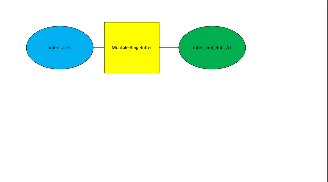
Figure 8: Data Flow Model from Section 2 of Part 2

Sources:
Michigan Department of Natural Resources (DNR)
ESRI
Price, Maribeth.2016. Mastering ArcGIS. 7th Edition data. McGraw Hill.
Wilson, Cyril 2012, A comprehensive Lake featres for Wisconsin

GIS Lab 4

GIS Lab 4

Goal and Background:
The goal for this lab was to be able to better develop our skills of composing query expressions to extract specific data from the databases we were provided with. We were to compose five different multiple criteria queries over the course of this lab, each of which would assess our knowledge of attribute and spatial queries and how to assess the results that come from the two.

Methods:
To begin, I started with a blank map and added the counties data located in USA mgisdata. For the first question I wrote a multiple criteria query from counties with a population between 3000 and 4000 people in 2010 and also all counties in 2010 that had a population density of at least 1000 persons per square mile. My query for this is demonstrated in Figure 1. I got this because if you want all of the population between 3000 and 4000 and also all of the counties that had a population density of at least 1000 person per square mile you use OR and not AND. To answer how many counties met the above criteria, how many states me the criteria above, which state has the highest number of counties, and which state had 8 counties that met the criteria; I used the information in the attribute table I got from doing the query itself. From there I created a cartographically pleasing map to show the results from that query.

Figure 1: Multiple criteria query for Question 1

For question 2 I wrote a multiple criteria query for counties in Wisconsin, Texas, New York, Minnesota, and California where the male population is greater than the female population and also for these states where the number of seniors is above 6500. The query I wrote is in Figure 2 below. I got this because it asked for all of the states so I put OR in between all of the states names, and then AND in between the other information because we just want the data that overlaps the counties in those particular states. I then used the attribute table from counties that I got from the query to answer the specific questions the records. And then, created a cartographically pleasing map shows the counties that the query represented.

Figure 2: Multiple criteria query for Question 2

For question 3 I wrote a multiple criteria query developed from the second question just modified. What was added to this query was all other seniors in Washington, Maryland, Illinois, Nebraska, District of Columbia, and Michigan who reside in counties that have more than 30,000 housing units. The resulting query is shown in Figure 3 and 3.1. This was modified from the query in question two by moving senior age range to the top, followed by the original states, then males greater than females which were all combined by AND, then I followed that with OR and the new housing unit information and the new states added in this question. After finishing the query I again used the attribute table in counties to answer the new question from this query, and then made a cartographically pleasing map to show the new query.

Figure 3: First part of query for Question 3

Figure 3.1: Second part of query for Question 3

In part 2 I first had to download and unzip the Wisconsin Data set information provided to us by Dr. Cyril Wilson to be able to work on questions four and five. For question 4 I wrote a query for cities in Wisconsin with a 2007 population between 15,000 and 20,000, area of the city is at least 5 square miles in land area and also female population is greater than males, and also the cities are within 2 miles of a lake. The result of this query is in figure 4 below. I did AND in between all of the information because we just wanted the data that crossed over all of it. You can't do an attribute query for distance from a lake, so for that I did a spatial query shown in figure 4.1 below. I then was able to answer the following questions from the attribute table and spatial query, and then again created a cartographically pleasing map of the cities that were recorded. 

Figure 4: Multiple criteria query for Question 4

Figure 4.1: Spatial query for Question 4

Finally, for question 5 I created a multiple criteria query from the following rivers in Wisconisn; Chippewa, Eau Claire, Embarrasss, Fisher, Hunting, Kinnickinnic, Maunesha, Milwaukee, Moose, Namekagon, Pelican, Platte, and Potato. The results are in Figures 5 and 5.1. Then in order to answer the questions about the records which included the total length of the the record of rivers from the query I had to create a new field in the Rivers attribute table. I then in that new field calculated the geometry in miles, and checked the Statistics bottom after to find the sum length in miles of all the rivers. Then created one last map of the resulted records found by this query.

Figure 5: Start of query for Question 5

Figure 5.1: End of query for Question 5

Results: In this results section I will be showing the final cartographically pleasing maps that are a result of the multiple criteria queries.

Figure 1.1: Map of query from question 1

Figure 2.1: Map of query from Question 2

Figure 3.2: Map of query from Question 3

Figure 4.2: Map of query from Question 4

Figure 5.2: Map of query from Question 5

Sources:
USA geodatabase data from the mgisdata from the Price book
Wisconsin cities, interstates, rivers, and counties shape files are from ESRI, 2011
Wisconsin Lakes created by Dr. Wilson 2012

GIS Lab 3

GIS Lab 3

Goal and Background:
        The goal of this lab was to familiarize ourselves with using standalone table data to map and analyze for GIS projects. More specifically to be able transform standalone tables into attribute tables with other data to be able to map the data together. Another goal was to be able to us the U.S. Census Bureau to get data and use that data for out GIS maps, and also to be able to familiarize ourselves with creating static and dynamic/web maps.

Methods:
        To begin, I downloaded the data from the U.S, Census Bureau of the total population of all Wisconsin counties from 2010 from the data set 2010 SFI 100% data unzipped it and saved it into my personal Lab 3 folder. I then went into the excel spreadsheet provided in the data (DEC_10_SFI_P1_with_ann.csv) and changed the last column title to Pop_2010, formatted the number cells to 0 for all the data in that column, then saved the file to Excel Workbook. I then went back online to the U.S. Census page and downloaded the map shape file for Wisconsin and unzipped and saved it in my personal Lab 3 folder as well. From there I opened up a new ArcMap and added the excel file and shape file I had downloaded. I then joined the excel file to the shape file of Wisconsin through GEO_ID and GE0#id then exported that to a new shape file. Then I removed the other data besides the new shape file from the Table of Contents. To make the map into what is shown in Figure 1, I went into symbology tab in the properties of the new shape file and changed the quantities (graduated colors) to make the counties different colors for the density of the populations. To finish it I made the map topographically pleasing by adding a title, north face, legend, and others.
       Next, I did the same exact thing as I described above except I used a different variable this time I used the Housing Units 2010 SFI 100% data from all the counties in Wisconsin from the U.S. census bureau online. After following those exact same steps I ended up with two static maps looking similar, but with different variables.
      After that, I created a dynamic/web map from the Housing Unit static map I previously created. I signed into ArcGIS online through the UWEC Geography and Anthropology Organization account. Then I was able to share my map online. I changed it's service name, changed the map to feature access, filled out an item description for the map, analyzed the map for any errors, and shared it with the account I created through UWEC in ArcGIS online. Then I went to the my content section of ArcGIS online added the layer I made into a new map. To finish it up I configured pop-ups for the counties so that when you click on a county on the map the name and data only for that county would show up. My map was finished, so I added again a final item description and shared the final map with the same Geography and Anthropology account.

Results: Figure 1 represents the data of housing units in all Wisconsin counties in 2010 I obtained from the U.S. Census Bureau that I joined with a shape file of the state of Wisconsin and made into a static map. Figure 2 represents the data of population density in all Wisconsin counties in 2010 that I also obtained from the U.S. Census Bureau and joined with a shape file of Wisconsin and made into a static map. Figure 3 represents the dynamic/web map I made from ArcGIS online from the static map of housing units static map I made prier.

Figure 1: Static map of the density of housing units in Wisconsin counties in 2010 

Figure 2: Static map of the population density of Wisconsin counties in 2010

Figure 3: Dynamic/web map of the housing units in Wisconsin counties in 2010

Sources: United States Census Bureau american fact finder 2010 database [March 8th, 2017]

ArcGIS Online Esri 

Lab 1

GIS Lab 1

Goal and Background:
        The goal of this Lab exercise was to be able to apply our knowledge learned in lecture and lab on geographic coordinate systems and projected coordinate systems to. Mostly to demonstrate our understanding of the differences between geographic and projected coordinate systems, and how to apply them to the GIS data in an appropriate format. Additional goals of this lab were to be able to correctly identify errors in the projections of GIS data and therefore be able to project or re-project them in a way they are usable in GIS. 

Methods:
          To begin this from the WORLD sub-folder I added the layers country and geog-rid to ArcMap and changed the legends on each shape-file. Then I applied the appropriate projection provided by the lab instructions, GCS -World- WGS 1984, to the same shape-files by going to the layers properties coordinate system tab. In separate data frame I then applied this for the next three changing the projections to the one provided (In order PCS- World- Mercator(world), PCS- World- Sinusoidal), and PCS- World- Equidistant Conic). Then for the fifth and last choose my own projection as directed which I went with PCS- World- Robinson.
          Then, still in the same Arcmap just another data frame, I inserted the states shape-file from the USA sub-folder. I then selected Wisconsin by going to select attributes and exported Wisconsin to its own shape-file. Like for the world maps I changed the symbolization and coordinate system to UTM, NAD 1983, Zone 16N.
          Again, I created a new data frame and then added the states shape-file and the stroads_miv5a shape-file from the USA sub-folder. There was a problem with the projections, so I needed to the tool box go to Data Management-Projections and Transformations-Feature-Project and go to the Project tool. I inputted the stroads_miv5a.shp file and then applied the states.shp file to make them both the same projection which is PCA-Continental-North America-North American Lambert Conformal Conic.I then arranged all of these 7 maps on the layout view with labels and other components thinking about cartography.
         Lastly, in a new ArcMaps I added the shape-file Central_WI_Cts.shp. There was an unidentified projection, so I changed the coordinate system by going to the tab in properties to GCS: North America_1983 and fixed the projection by going to the projection tool in the tool box and changing it to the PCS-State Plane-Wisconsin Central. Then I brought in the shape-file Lower_Chip_strms.shp. The projection didn't fit with that of the last shape-file, so again I went into the projection tool and changed it to match which was PCS-State Plane-Wisconsin Central. Then putting it in layout view I added labels and components.

Results: Figure 1 shows the multiple world map projection coordinate systems I talked about before, the Wisconsin UTM projection, and the States projection matched up with the roads shape-file all in a layout view. Figure 2 shows  central Eau Claire county and the counties surrounding it with the rivers showing the fixed projections of the shape-files. 

Figure 1. These are the images of the map projections demonstrated in Lab 1. 

Figure 2. This is the map showing the projection changes for Eau Claire and surrounding counties

Sources: Database from Dr. Cyril Wilson database folder Lab1_data.zip